LLM(二)——Attention机制

Attention 机制很像人类看图片的逻辑，当我们看一张图片的时候，我们并没有看清图片的全部内容，而是将注意力集中在了图片的焦点上。我们的视觉系统就是一种 Attention机制，将有限的注意力集中在重点信息上，从而节省资源，快速获得最有效的信息。

seq2seq

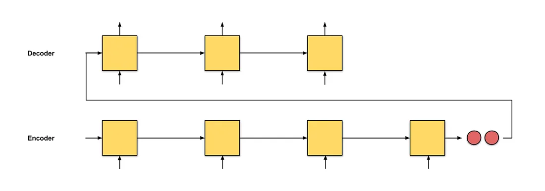
在seq2seq中，有一个Encoder和一个Decoder，Encoder和Decoder都是RNN。seq2seq的缺点在于Decoder从Encoder接收的唯一信息就是最后Encoder隐藏状态(上图红色点)。如果输入文本很长，仍然使用定长向量来表示句子的信息，这会导致部分信息的丢失。

Attention的想法基础就是在把原先输入Decoder的定长向量，改为对Encoder的输出向量加权和的形式，这个加权和的计算过程就叫Attention。

一、Attention机制概述

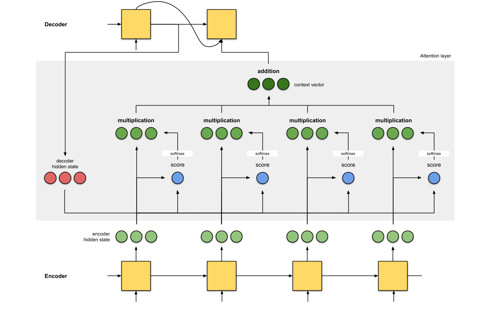
通过为每个单词分配一个权重，注意力机制能够为当前翻译的单词对原文各个单词计算出不同的权重以实现关注点的不同。由于这个权重可能大于1，所以使用softmax进行归一化，得到归一化权重，然后计算Encoder隐藏状态和其对应归一化权重的加权和，得上下文向量。

计算分数

利用Encoder所有的隐藏状态和Decoder的第一个隐藏状态。要想输出Decoder的第一个隐藏的状态，需要给Decoder一个初始状态和一个输入，例如采用Encoder的最后一个状态作为Decoder的初始状态，输入为0。计算Decoder的第一个隐藏状态和Encoder所有的隐藏状态的相关性，这里采用点积的方式。

每个Encoder隐藏状态乘以其softmax得分

把得到的分数输入到到softmax层，进行归一化，归一化后的分数代表的注意分配的权重。将每个Encoder隐藏状态与其softmax得分（标量）相乘。

加权求和，并将向量送入Decoder

将上述加权后的向量求和，得到上下文向量。上下文向量就是对所有隐藏状态的向量进行信息聚合。然后将上下文向量输入到Decoder中。

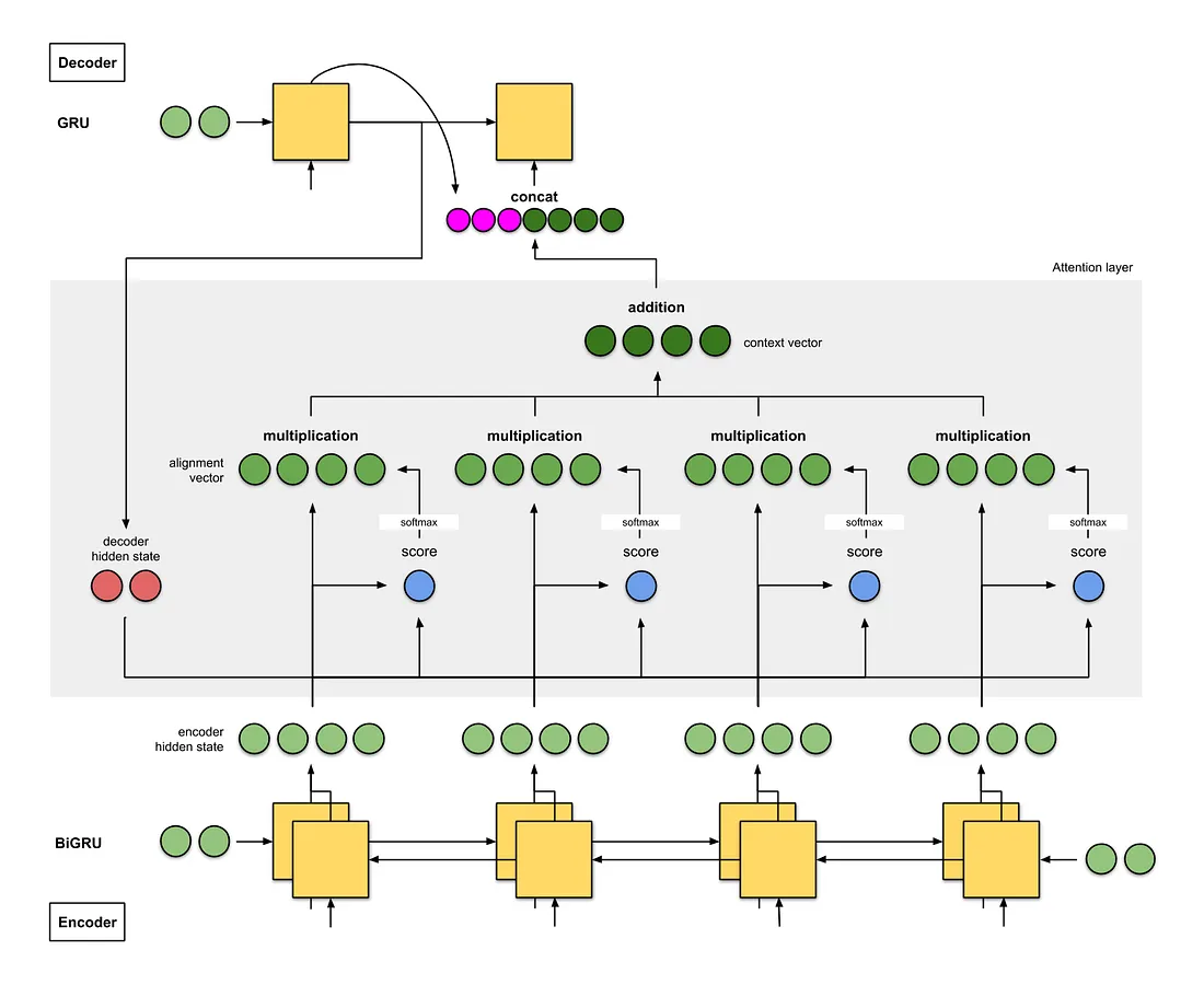
Bahdanau注意力 ^[1]

• Encoder是双向（前向+后向）门控循环单元（BiGRU）。
• Decoder是GRU，其初始隐藏状态来自EncoderGRU的最后隐藏状态向量。
• 注意层中的评分方法是点积加权和，下一个Decoder时间步的输入是来自前一个Decoder时间步（粉红色）的输出和当前时间步（深绿色）的上下文向量之间的拼接（concat）。

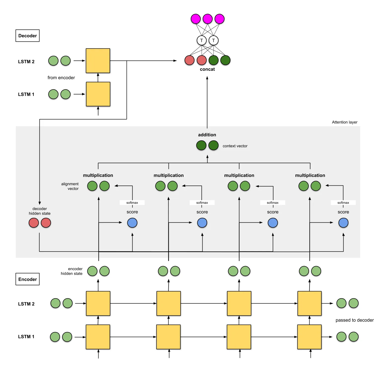
Luong注意力 ^[2]

• Encoder是两层的LSTM网络。 Decoder也一样，其初始隐藏状态是最后Encoder隐藏状态。
• 实验的评分函数是（i）add和concat，（ii）dot，（iii）location，和（iv）general。
• 拼接得到的上下文向量输入一个前馈神经网络得到的输出（粉红色）作为当前Decoder时间步的输入。

二、Attention 的原理

Attention 并不一定要在 Encoder-Decoder 框架下使用的，他是可以脱离 Encoder-Decoder 框架的。比较主流的attention框架如下：

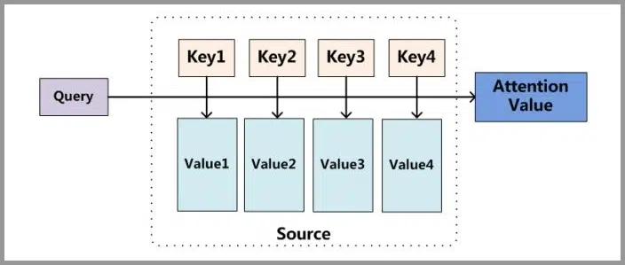
将Source中的元素想像成一系列的<Key,Value>数据对，此时指定Target中的某个元素Query，通过计算Query和各个元素相似性或者相关性，得到每个Key对应Value的权重系数，然后对Value进行加权求和，得到最终的Attention值。

本质上Attention机制是对Source中元素的Value值进行加权求和，而Query和Key用来计算对应Value的权重系数。

Attention 原理的3步分解：

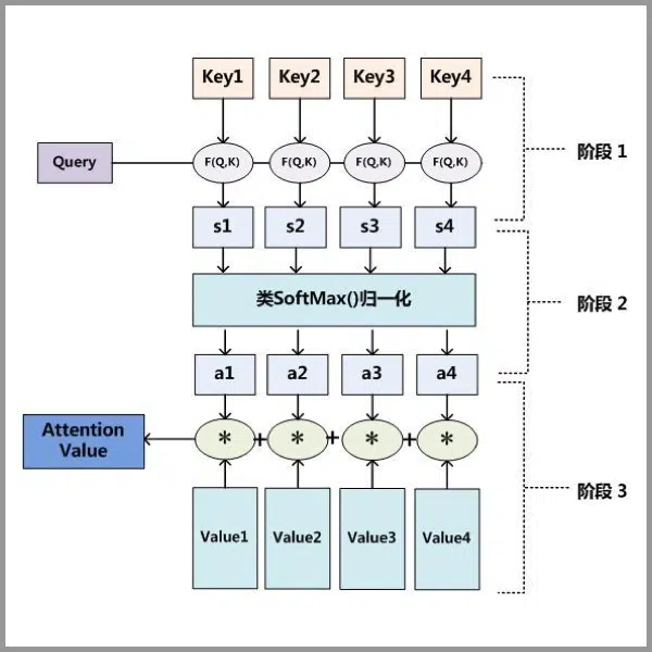
1. Query与Key进行相似度计算得到权值
2. 对上一阶段的计算的权重进行归一化
3. 用归一化的权重与Value加权求和，得到Attention值

一个简单的例子：

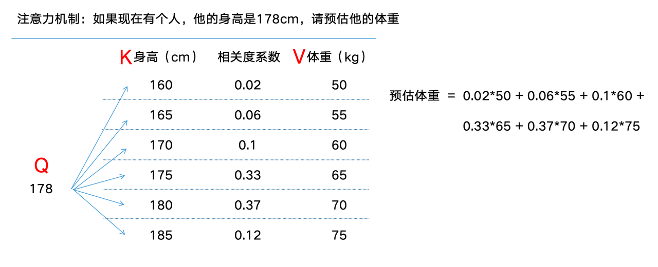
Q,K,V都会被向量化，先拿Q与所有K进行向量点积（或其他计算分数的公式），然后softmax求得相识度分数，最后用分数对结果进行加权求和，得到结果向量，然后转换成最终结果。

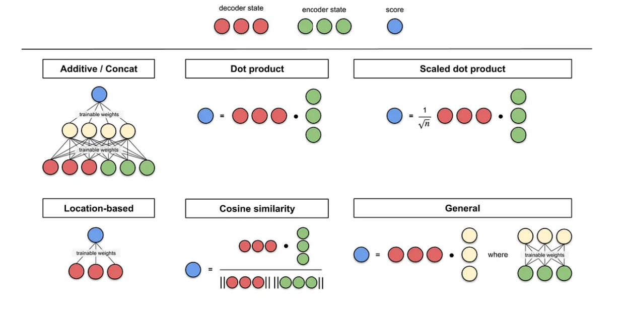
三、注意力评分函数

Q,K间的分数计算函数可以视为注意力评分函数（attention scoring function），简称评分函数（scoring function），然后把这个函数的输出结果输入到softmax函数中进行运算。通过上述步骤，将得到与键对应的值的概率分布（即注意力权重）。最后，注意力汇聚的输出就是基于这些注意力权重的值的加权和。

下图说明了如何将注意力汇聚的输出计算成为值的加权和，其中表示注意力评分函数。由于注意力权重是概率分布，因此加权和其本质上是加权平均值。

用数学语言描述，假设有一个查询和个“键－值”对，其中，。注意力汇聚函数就被表示成值的加权和：

其中查询和键的注意力权重（标量）是通过注意力评分函数将两个向量映射成标量，再经过softmax运算得到的：

正如上图所示，选择不同的注意力评分函数会导致不同的注意力汇聚操作。

3.1 masked softmax

在文本翻译中为了高效处理小批量数据集， 某些文本序列被填充了没有意义的特殊词元。为了仅将有意义的词元作为值来获取注意力，可以指定一个有效序列长度（即词元的个数），以便在计算softmax时过滤掉超出指定范围的位置。

import math
import torch
from torch import nn

def sequence_mask(X, valid_len, value=0):
    """在序列中屏蔽不相关的项"""
    maxlen = X.size(1)
    mask = torch.arange((maxlen), dtype=torch.float32,
                        device=X.device)[None, :] < valid_len[:, None]
    X[~mask] = value
    return X

def masked_softmax(X, valid_lens):
    """通过在最后一个轴上掩蔽元素来执行softmax操作"""
    # X:3D张量，valid_lens:1D或2D张量
    if valid_lens is None:
        return nn.functional.softmax(X, dim=-1)
    else:
        shape = X.shape
        if valid_lens.dim() == 1:
            valid_lens = torch.repeat_interleave(valid_lens, shape[1])
        else:
            valid_lens = valid_lens.reshape(-1)
        # 最后一轴上被掩蔽的元素使用一个非常大的负值替换，从而其softmax输出为0
        X = sequence_mask(X.reshape(-1, shape[-1]), valid_lens,
                              value=-1e6)
        return nn.functional.softmax(X.reshape(shape), dim=-1)

3.2 additive attention

当查Q和K是不同长度的矢量时，可以使用加性注意力作为评分函数。给定查询和键，加性注意力（additive attention）的评分函数为

其中可学习的参数是、和。将查询和键连结起来后输入到一个多层感知机（MLP）中，感知机包含一个隐藏层，其隐藏单元数是一个超参数。通过使用作为激活函数，并且禁用偏置项。

class AdditiveAttention(nn.Module):
    """加性注意力"""
    def __init__(self, key_size, query_size, num_hiddens, dropout, **kwargs):
        super(AdditiveAttention, self).__init__(**kwargs)
        self.W_k = nn.Linear(key_size, num_hiddens, bias=False)
        self.W_q = nn.Linear(query_size, num_hiddens, bias=False)
        self.w_v = nn.Linear(num_hiddens, 1, bias=False)
        self.dropout = nn.Dropout(dropout)

    def forward(self, queries, keys, values, valid_lens):
        queries, keys = self.W_q(queries), self.W_k(keys)
        # 在维度扩展后，
        # queries的形状：(batch_size，查询的个数，1，num_hidden)
        # key的形状：(batch_size，1，“键－值”对的个数，num_hiddens)
        # 使用广播方式进行求和
        features = queries.unsqueeze(2) + keys.unsqueeze(1)
        features = torch.tanh(features)
        # self.w_v仅有一个输出，因此从形状中移除最后那个维度。
        # scores的形状：(batch_size，查询的个数，“键-值”对的个数)
        scores = self.w_v(features).squeeze(-1)
        self.attention_weights = masked_softmax(scores, valid_lens)
        # values的形状：(batch_size，“键－值”对的个数，值的维度)
        return torch.bmm(self.dropout(self.attention_weights), values)

3.3 scaled Dot-Product attention

使用点积可以得到计算效率更高的评分函数，但是点积操作要求查询和键具有相同的长度。假设查询和键的所有元素都是独立的随机变量，并且都满足零均值和单位方差，那么两个向量的点积的均值为，方差为。为确保无论向量长度如何，点积的方差在不考虑向量长度的情况下仍然是，将点积除以，则缩放点积注意力（scaled dot-product attention）评分函数为：

在实践中，通常从小批量的角度来考虑提高效率，例如基于个查询和个键－值对计算注意力，其中查询和键的长度为，值的长度为。查询、键和值的缩放点积注意力是：

缩放因子的作用

缩放因子的作用是归一化:

假设,里的元素的均值为0，方差为1，那么中元素的均值为0，方差为d，标准差是。 当d变得很大时， 中的元素的方差也会变得很大，如果中的元素方差很大，那么的分布会趋于陡峭(分布的方差大，分布集中在绝对值大的区域)。总结一下就是的分布会和d有关。因此中每一个元素除以后，方差又变为1,这将使得近似服从标准正态分布。这使得的分布“陡峭”程度与d解耦，从而使得训练过程中梯度值保持稳定。

class DotProductAttention(nn.Module):
    """缩放点积注意力"""
    def __init__(self, dropout, **kwargs):
        super(DotProductAttention, self).__init__(**kwargs)
        self.dropout = nn.Dropout(dropout)

    # queries的形状：(batch_size，查询的个数，d)
    # keys的形状：(batch_size，“键－值”对的个数，d)
    # values的形状：(batch_size，“键－值”对的个数，值的维度)
    # valid_lens的形状:(batch_size，)或者(batch_size，查询的个数)
    def forward(self, queries, keys, values, valid_lens=None):
        d = queries.shape[-1]
        # 设置transpose_b=True为了交换keys的最后两个维度
        scores = torch.bmm(queries, keys.transpose(1,2)) / math.sqrt(d)
        self.attention_weights = masked_softmax(scores, valid_lens)
        return torch.bmm(self.dropout(self.attention_weights), values)

注意力评分函数总结图

四、Bahdanau注意力代码实现

所依赖函数在之前RNN以及更多RNN章节中包含

注意力解码器

class AttentionDecoder(Decoder):
    """带有注意力机制解码器的基本接口"""
    def __init__(self, **kwargs):
        super(AttentionDecoder, self).__init__(**kwargs)

    @property
    def attention_weights(self):
        raise NotImplementedError

实现带有Bahdanau注意力的循环神经网络解码器

首先，初始化解码器的状态，需要下面的输入：

1. 编码器在所有时间步的最终层隐状态，将作为注意力的键和值；
2. 上一时间步的编码器全层隐状态，将作为初始化解码器的隐状态；
3. 编码器有效长度（排除在注意力池中填充词元）。

class Seq2SeqAttentionDecoder(AttentionDecoder):
    def __init__(self, vocab_size, embed_size, num_hiddens, num_layers,
                 dropout=0, **kwargs):
        super(Seq2SeqAttentionDecoder, self).__init__(**kwargs)
        self.attention = AdditiveAttention(
            num_hiddens, num_hiddens, num_hiddens, dropout)
        self.embedding = nn.Embedding(vocab_size, embed_size)
        self.rnn = nn.GRU(
            embed_size + num_hiddens, num_hiddens, num_layers,
            dropout=dropout)
        self.dense = nn.Linear(num_hiddens, vocab_size)

    def init_state(self, enc_outputs, enc_valid_lens, *args):
        # outputs的形状为(batch_size，num_steps，num_hiddens).
        # hidden_state的形状为(num_layers，batch_size，num_hiddens)
        outputs, hidden_state = enc_outputs
        return (outputs.permute(1, 0, 2), hidden_state, enc_valid_lens)

    def forward(self, X, state):
        # enc_outputs的形状为(batch_size,num_steps,num_hiddens).
        # hidden_state的形状为(num_layers,batch_size,
        # num_hiddens)
        enc_outputs, hidden_state, enc_valid_lens = state
        # 输出X的形状为(num_steps,batch_size,embed_size)
        X = self.embedding(X).permute(1, 0, 2)
        outputs, self._attention_weights = [], []
        for x in X:
            # query的形状为(batch_size,1,num_hiddens)
            query = torch.unsqueeze(hidden_state[-1], dim=1)
            # context的形状为(batch_size,1,num_hiddens)
            context = self.attention(
                query, enc_outputs, enc_outputs, enc_valid_lens)
            # 在特征维度上连结
            x = torch.cat((context, torch.unsqueeze(x, dim=1)), dim=-1)
            # 将x变形为(1,batch_size,embed_size+num_hiddens)
            out, hidden_state = self.rnn(x.permute(1, 0, 2), hidden_state)
            outputs.append(out)
            self._attention_weights.append(self.attention.attention_weights)
        # 全连接层变换后，outputs的形状为
        # (num_steps,batch_size,vocab_size)
        outputs = self.dense(torch.cat(outputs, dim=0))
        return outputs.permute(1, 0, 2), [enc_outputs, hidden_state,
                                          enc_valid_lens]

    @property
    def attention_weights(self):
        return self._attention_weights

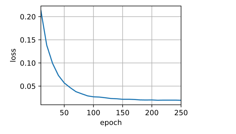
训练

embed_size, num_hiddens, num_layers, dropout = 32, 32, 2, 0.1
batch_size, num_steps = 64, 10
lr, num_epochs, device = 0.005, 250, try_gpu()

train_iter, src_vocab, tgt_vocab = load_data_nmt(batch_size, num_steps)
encoder = Seq2SeqEncoder(
    len(src_vocab), embed_size, num_hiddens, num_layers, dropout)
decoder = Seq2SeqAttentionDecoder(
    len(tgt_vocab), embed_size, num_hiddens, num_layers, dropout)
net = EncoderDecoder(encoder, decoder)
train_seq2seq(net, train_iter, lr, num_epochs, tgt_vocab, device)

loss 0.019, 25753.3 tokens/sec on cuda:0

预测

engs = ['go .', "i lost .", 'he\'s calm .', 'i\'m home .']
fras = ['va !', 'j\'ai perdu .', 'il est calme .', 'je suis chez moi .']
for eng, fra in zip(engs, fras):
    translation, dec_attention_weight_seq = d2l.predict_seq2seq(
        net, eng, src_vocab, tgt_vocab, num_steps, device, True)
    print(f'{eng} => {translation}, ',
          f'bleu {d2l.bleu(translation, fra, k=2):.3f}')

go . => va !,  bleu 1.000
i lost . => j'ai perdu .,  bleu 1.000
he's calm . => il est riche .,  bleu 0.658
i'm home . => je suis chez moi .,  bleu 1.000

参考

1. Attn: Illustrated Attention
2. 图解Attention
3. Attention 机制
4. Attention机制的基本思想与实现原理
5. 李沐-动手学深度学习第二版
6. 为什么attention计算要除根号d
7. Attention Is All You Need

1. https://arxiv.org/pdf/1409.0473 ↩︎
2. https://arxiv.org/pdf/1508.04025
   ↩︎